Break adjusted levels
These Explanatory notes use the term break-adjusted to relate to amounts outstanding (levels) data series constructed to be consistent with transactions (flows) and growth rates data. The term break-adjusted is not applied to flows and growth rates data, as it is understood that these data, by definition, incorporate any adjustments required to offset the impacts of breaks.
With the exception of a limited number of high profile monetary aggregates series, the Bank of England does not routinely publish data for break-adjusted levels series. Other than for these exceptions, Bank of England published levels data should be understood to be non-break-adjusted. One reason for this approach is to avoid a potential source of confusion to users, given that any break-adjusted levels series can be arbitrarily scaled. Data users can, however, readily construct break-adjusted series consistent with the published data for themselves. This is explained below.
Break-adjusted levels data can be constructed by fixing the level for any arbitrarily chosen reference period, and recursively dividing (or multiplying) by one-period growth rate factors to generate values for all other periods in the range of interest, before (or after), the reference period. The growth rate factor is determined from the flow during the period and the amount outstanding at the previous period. One option is to choose the reference period to represent the latest published data point. In this case, the break-adjusted amount outstanding in the reference period is the value of the published amount outstanding, and levels for all preceding periods are calculated by successively dividing by the growth rate factors. Another approach can be to choose a historic reference period and to take the published value for that period, or to set it to 100 in order to create break-adjusted series in index form, and then to apply growth rate factors to subsequent and preceding periods as appropriate.
If break-adjusted versions of both seasonally-adjusted (SA) and non-seasonally adjusted (NSA) forms of a data series are to be constructed, users may wish to ensure that seasonal adjustment factors are preserved in the constructed series (or index). To do this, it is sufficient to constrain the reference period values of the break-adjusted SA and NSA series to be the corresponding values of the published data in that period.
For a break-adjusted series expressed in index form, it would be necessary to ensure that the ratio of the SA and NSA versions of the index series equates to the seasonal factor, that is to the ratio of the SA and NSA forms of the non-break adjusted data, in all periods. This can be achieved by setting the break-adjusted NSA and SA index values in the reference period to 100, and 100 x the reference period seasonal factor, respectively.
Break-adjusted formulae
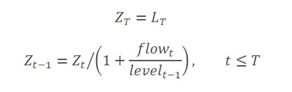
The following formulae illustrate the calculation of break-adjusted data in terms of flows and preceding period levels. In this example, the reference period is the latest available period, T. First, the break-adjusted levels series, Z, is set equal to the published value, L, for the amount outstanding in the reference period, t=T. Break-adjusted levels for preceding periods are defined recursively:
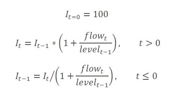
For the case of a break-adjusted series expressed as an index, suppose that the index level may be written asI in period t, where I=100in the reference period t=0. Subsequent (and preceding) values are calculated by compounding growth rate factors (forwards or backwards, as required). In terms of the current period flow and the previous period amount outstanding, these expressions may be written as:
Alternative formulae
In the above expressions, it might be considered more straightforward simply to substitute the growth rate into the growth rate factors, rather than to express these in terms of the ratio of the flow to the previous period amount outstanding. Mathematically this would be an equivalent definition, and would reflect an understanding that the break-adjusted data series contains the same information as the growth rates data in combination with a scaling of the data. However, the approach given above is suggested on account of the fact that Bank of England growth rates data are published (and held) to one decimal place in percentages, and users may prefer to compute break-adjusted data to a greater degree of precision, comparable with that of the amounts outstanding data.
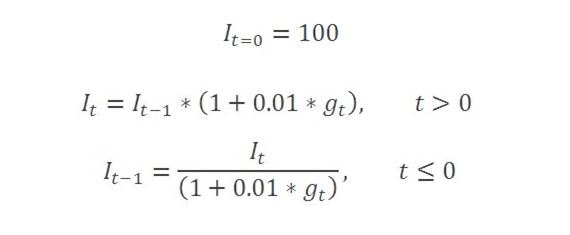
For completeness, the alternative calculation based directly on percentage growth rates, g, would be written as follows:
As noted, if the growth rates data are held to a lower degree of precision than the underlying flows and amounts outstanding, then performing the calculation of break-adjusted amounts outstanding in this way will introduce rounding errors in each period. These would affect the precision both of the amounts outstanding and any implied growth rate calculations. For example, the implied 12-month growth rate of a break-adjusted amounts outstanding series, calculated from percentage growth rates data held to one decimal place, would have a rounding error with standard deviation of 0.1 percentage points.
Worked example
These calculations are illustrated in spreadsheet format in this worked example.